| Output from the INMOS distributed Z-buffer system | |
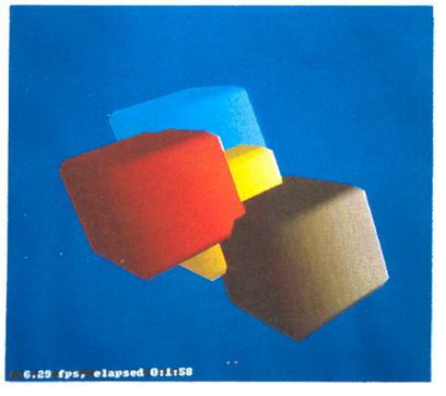
| Four
intersecting cubes
|
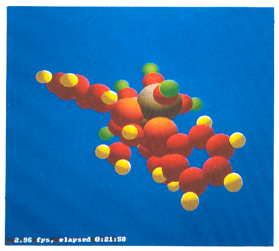
A simple
molecule
|
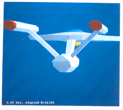
| The
Starship Enterprise
|
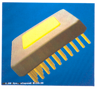
The IMS
T800 package
|
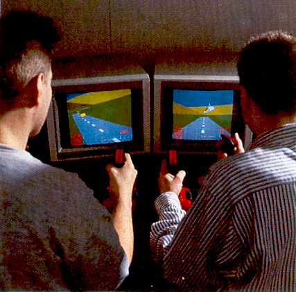
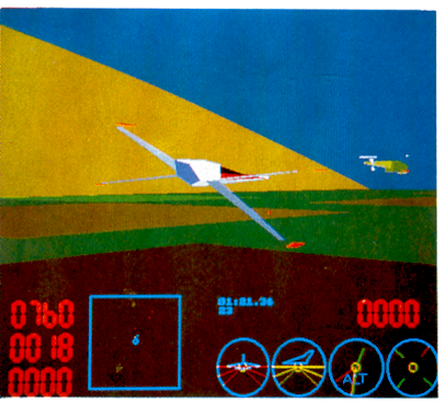
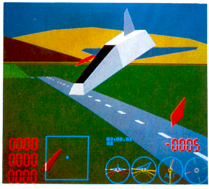
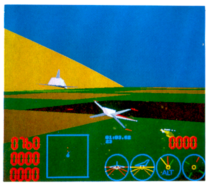
| Output from the INMOS multiplayer flight simulator | |
 |
 |
 |
 |
1 Introduction
2 Computer graphics techniques
2.1 Modelling objects
2.2 Transformation2.2.1 The homogenous coordinate system
2.2.2 Translation
2.2.3 Rotation
2.2.4 Concatenation
2.2.5 Perspective projection2.3 Scan conversion
2.4 Shading
2.5 Clipping
2.6 Hidden surface removal
3 The IMS T800 transputer
3.1 Serial links
3.2 On-chip floating point unit
3.3 2-D block move instructions
3.4 The occam programming language
3.5 Meeting computer graphics requirements
4 3-D transformation on the IMS T800
5 The INMOS distributed Z-buffer
5.1 The Z-buffer algorithm
5.2 Scan conversion
5.2.1 Scan converting polygons
5.2.2 Scan converting spheres
5.2.3 Implementation detailsScan conversion with a DDA
Scan conversion on transputers5.2.4 Distributing scan conversion over multiple transputers
5.3 Architecture
5.4 Performance
6 The INMOS multi-player flight simulator
6.1 Requirements
6.2 Implementation details
6.2.1 The distributed polygon shader
6.2.2 Geometry system
6.2.3 BSP-trees6.3 Architecture
6.4 Performance
7 Conclusions
This technical note examines some applications of the IMS T800 floating point transputer in high performance graphics systems. Firstly there is a brief introduction to some of the the basic techniques and terminology used in computer graphics. This includes comments on implementation and processing requirements.
Section 3 provides an overview of transputer, and specifically IMS T800, architecture. This concentrates on the aspects of the device which make it particularly suitable for using in parallel graphics systems. There is also a brief description of the occam language, designed for programming highly parallel systems. This part concludes with a summary of how the IMS T800 meets the requirements of a modern graphics system.
The next section describes in some detail how the computing performance of the floating point processor is obtained. It uses, as an example, a procedure which forms one of the key routines in all our graphics demonstrations.
Finally two particular applications are described in detail. These are the INMOS distributed Z-buffer, a near real time multiprocessor solution to the hidden surface problem, and the INMOS multi-player flight simulator, a real time interactive combat simulator. Both programs have been implemented on standard INMOS transputer evaluation boards with no custom hardware design and written entirely in a high level programming language.
Computer generated images, and in particular interactive graphics, is one of the fastest growing and most important application areas for high performance computing systems. Some common applications are computer aided design (CAD), simulation and medical imaging. These allow the user to rapidly see the effects of, for example, a design change on the appearance or behaviour of an object; or to view a large amount of data (for example a three dimensional scan of a human body) in an understandable form.
There are a number of common requirements for these systems. Firstly the system must be fast, both to generate an image and to respond to input from the user. Secondly the displayed images must be realistic, or at least readily comprehensible to the user. This will usually mean that objects can be viewed with correct perspective, with natural shading and possibly shadowing, and that the way in which one part of the scene obscures another (the ‘hidden surface problem’) is correctly represented. For interactive systems response speed is an important factor to maintain realism and usability.
A brief introduction to some of the techniques and terminology used in this paper is given below. A good introduction to interactive computer graphics can be found in [11].
In order to render or generate images of an object some way of modelling the object in the computer is needed. A convenient primitive to use as the basis of modelling objects is the polyhedron. By increasing the number of faces the shape of any solid object can be approximated, although at the cost of having more data to manipulate. An arbitrary polyhedron can be modeled by defining its faces; each of these faces is then a polygon which can be defined by an ordered list of vertex coordinates.
Each polygon will have other attributes associated with it, such as colour and orientation. The orientation is represented by a line or vector perpendicular to the surface. This is called the surface normal and can be calculated from the coordinates of three vertices. The surface normal is closely related to another attribute, the plane equation of the face. A plane is represented by four numbers (a, b, c, d) so that ax+ by + cz+ d = 0 is true only if the point [ x y z ] lies in the plane. If a point does not lie in the plane then the sign of the expression ax+by+cz+ d indicates which side of the plane the point is located on. By convention, points in front of the plane have positive values of ax+ by+ cz+ d. The components of the normal vector are given by the plane equation; the vector is [ a b c ]. The plane equation and normal vector are very important for visibility and shading calculations.
Geometric transformations play an important role in generating images of 3-dimensional scenes. They are used (a) to express the location and orientation of objects relative to one another and (b) to achieve the effect of different viewing positions and directions. Finally a perspective transformation is used to project the 3-dimensional scene onto a 2-dimensional display screen.
Transformations are implemented as matrices which are used to multiply a set of coordinates to give the transformed coordinates. All rotations, translations and other transformations to be performed on data are combined into a single matrix which can then be applied to each point being transformed. Transformations may be nested, like subroutine calls, so that parts of a model can be moved independently but still take on the global movement of the model or the viewpoint.
The coordinates of points are represented using what are known as homogenous coordinates. Any point in 3-dimensional space can be mapped to a point in 4-dimensional homogenous space. The fourth coordinate, w, is simply a scaling factor so a point with the homogenous coordinates [ x y z w ] is represented in 3-space as [ x/w y/w z/w ]. This representation simplifies many calculations and, in particular, means that the division required by perspective transformation can be done after clipping when there may be many fewer points to process.
The value of w is arbitrary as long as x, y, and z are scaled by the same amount. Generally when converting from 3-D to homogenous coordinates it is simplest to make w = 1 so no multiplication of x, y, and z is necessary. After being transformed the value of w may have changed so at some point the x, y, and z coordinates must be divided by w. This can be done when scaling to physical screen coordinates.
The transformation matrices used are 4x4 matrices for the transformation of homogenous coordinates and are designed to have the desired effect on the point in ordinary 3-space. When implemented on a computer, coordinates and transforms will generally use floating point representation for maximum accuracy and dynamic range.
Translation, or movement of a point in space, is simply achieved by adding the distance to be moved in each axis to the corresponding coordinate:
x' = x + tx
y' = y + ty
z' = z + tz
where tx, ty, and tz, are the distances moved in x, y and z respectively. This can be represented as a matrix multiplication:
[ x' y' z' ] = [ x y z ] |
|
|
|
|
|1 0 0 0 |
|
|
|
|
|0 1 0 0 0 0 1 0 tx ty tz 1
Three dimensional rotations can be quite complex. The simplest form is rotating a point about an axis which passes through the origin of the coordinate system, and is aligned with a coordinate axis. For example, rotation about the z axis by an angle of q is written as
x' =   x cos q + y sin q
y' = – x sin q + y cos q
This can be represented as a matrix multiplication as shown:
[ x' y' z' w' ] = [ x y z w ] |
|
|
|
|
|cos q -sin q 0 0 |
|
|
|
|
|sin q cos q 0 0 0 0 1 0 0 0 0 1
To perform rotations about an arbitrary point it is necessary to translate the point to the origin, perform the rotation and then translate the point back to its original position. Rotations about axes which are not aligned with the coordinate system can be performed by concatenating a number of simpler rotations.
The successive application of any number of transforms can be achieved with a single transformation matrix, the concatenation of the sequence. Suppose two transformations M1 and M1 are to be applied to successively to the point v. First v is transformed into v' by M1, this is then transformed into v" by M2:
v' = v M1 (2.1) v'' = v' M2 (2.2)
Substituting Equation 2.1 into Equation 2.2 gives:
v'' = (v M1) M2 = v (M1 M2)
Therefore the concatenation of a sequence of transformations is simply the product of the individual transform matrices. Note that, because matrix multiplication does not commute, the order of application of the transformations must be preserved.
| Figure 2.1: Viewing
objects in perspective
|
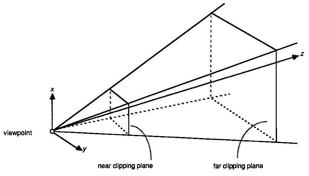
The most realistic way of displaying three dimensional objects on a two dimensional screen is the perspective projection. There is a simple transformation that distorts objects so that, when viewed with parallel projection (orthographically), they appear in perspective. This defines a viewing volume, a truncated pyramid, within which objects are visible (see Figure 2.1). This transformation preserves the flatness of planes and the straightness of lines and simplifies the clipping process that follows. The perspective transform uses three parameters: the size of the virtual screen onto which the image is projected; the distance from the viewing position to this screen; and the distance to the farthest visible point. The result of the perspective transform is to normalise all coordinates so that values range between -1 and +1, the centre of the image is at point (x, y) = (0, 0). To display these on a real device the coordinates must be scaled by the screen resolution of the display.
The perspective transform used in the programs discussed in this document is based on that in Sutherland and Hodgman [15].
Raster displays are the most commonly used output device for computer graphics systems. They represent an image as a rectangular array of dots or ‘pixels’. The image to be displayed is stored in a ‘frame buffer’, an area of memory where each location maps onto one pixel. The main advantages of raster displays are low cost and their ability to display solid areas of colour as easily as text and lines.
In order to display objects which are represented as a number of polygons it is necessary to scan convert the polygons. This involves finding all the pixels that lie inside the polygon boundaries and assigning them the appropriate colour. A shading model is used to calculate the colour of each pixel.
A number of techniques have been developed for scan conversion. These generally take advantage of ‘coherence’, the fact that the visibility and colour of adjacent pixels is usually very similar, there are only abrupt changes at polygon boundaries. This allows incremental methods using only integer arithmetic to be used.
To generate realistic images it is necessary to assign the correct colours to the various parts of the model. This means shading the objects to represent lighting conditions. The apparent colour of a surface is dependent on the nature of the surface (its colour, texture etc), the direction of the light source and the viewing angle. A realistic shading model may require a large amount of floating point arithmetic to multiply together the vectors representing surface orientation (the surface normal), direction of the light source etc.
Where objects are represented as a number of polygons, the faceted appearance can be reduced by using a smooth shading model. There are two simple and reasonably effective techniques. Gouraud shading simply interpolates the surface colour across each polygon. This can, however, introduce a number of anomalies for example, in the shape of highlights and the way shading changes in moving sequences. Many of these problems can be relieved by using a technique developed by Phong but at the expense of increased calculation. Phong shading interpolates the surface normals across the polygons and re-applies the shading model at each pixel.
Clipping is necessary to remove points which lie outside the viewing volume and to truncate lines which extend beyond the boundaries. Clipping can be done more simply after the perspective transformation. However, clipping in the z axis must be done before the division by depth which the full perspective projection requires as this destroys the sign information that determines whether a point is in front of or behind the viewer. Points with a negative value of z are behind the viewer.
Clipping to the x and y coordinates need only be performed to screen resolution. This has led to many clever, although not always simple, techniques using fast integer arithmetic to clip lines quickly. The availability of fast floating point hardware means that more straightforward methods can be used.
The use of homogenous coordinates and the perspective projection simplifies clipping. Because the points can be viewed in parallel projection x and y values which are inside the viewing pyramid are in the range -1 to 1 and z values are in the range 0 to 1. The use of scaled, homogenous coordinates means that the tests that have to be applied are:
–w <= x <= w
–w <= y <= w
 0 <= z <= w
These limits correspond to the six bounding planes of the truncated viewing pyramid. A fast polygon clipping algorithm is described in [15].
In order to generate realistic images it is important to remove from an image those parts of solid objects which are hidden. In real life these would be obscured by the opaque material of the object. In computer graphics the visibility of every point must be explicitly calculated.
Hidden surface algorithms are classified as either object-space or image-space. An object-space algorithm uses the geometrical relationships between the objects to determine the visibility of the various parts and so will normally require at least some floating point arithmetic. An image-space method works at the resolution of the display device and determines what is visible at each pixel. This can be done most efficiently using integer arithmetic. The computation time of object-space techniques tends to grow with the total number of objects in the scene whereas image-space computation will tend to grow with the complexity of the displayed image.
There is also a trade-off between speed, complexity and memory usage. For example the Z-buffer technique described in Section 5 is a very simple, reasonably fast image-space algorithm but requires a large amount of working memory. It uses an array of integers, the same size as the frame buffer, to store the depth at each pixel.
The BSP-tree used in the INMOS flight simulator (Section 6) is an object-space algorithm which is efficient in memory usage, but uses floating point arithmetic to determine the ordering of polygons. Its performance depends on the availability of a fast floating point processor. It is also not completely general: in its simplest form it can only be applied to rigid objects constructed from non-intersecting polygons.
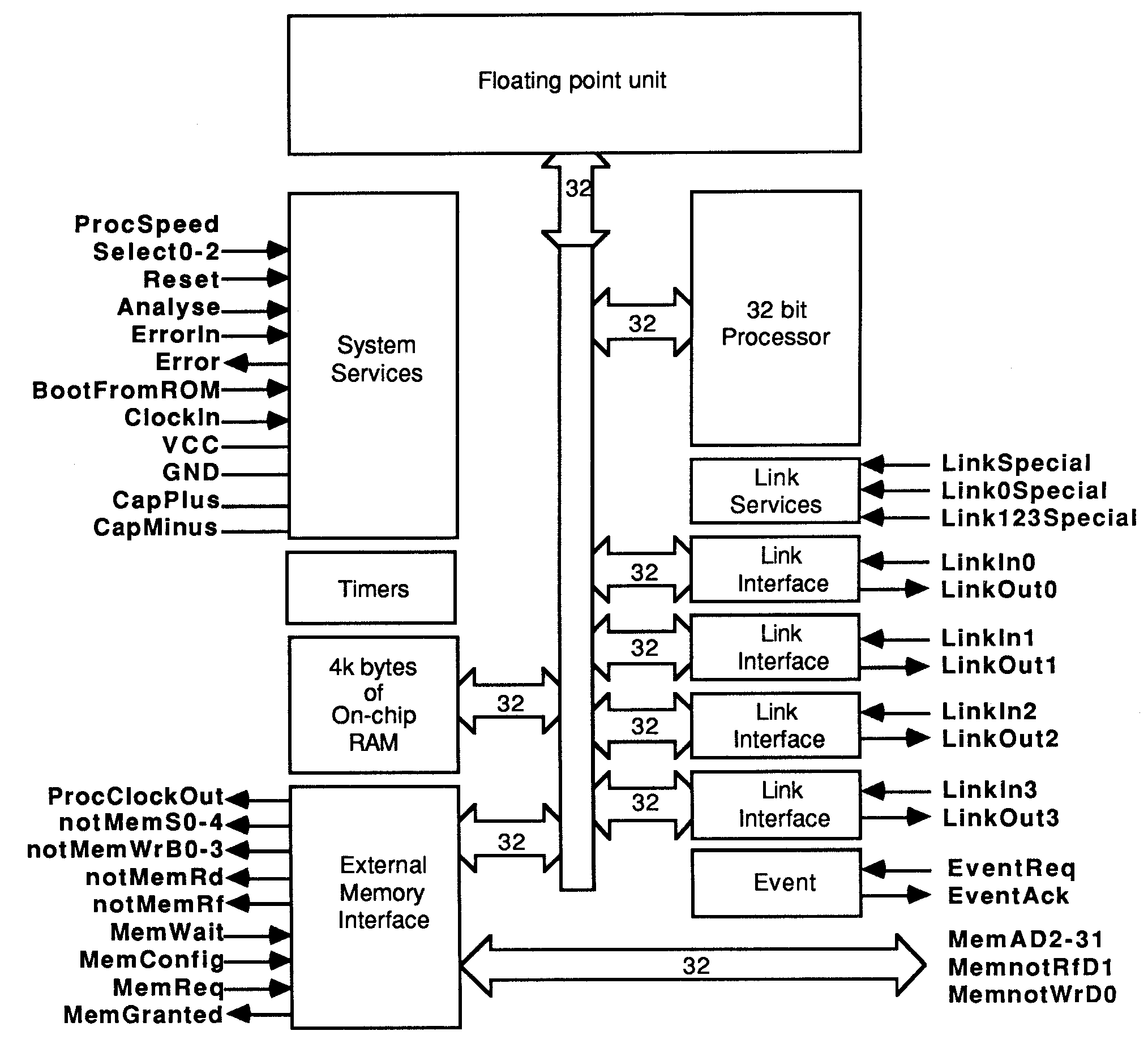
The IMS T800 is the latest member of the INMOS transputer family [1]. It integrates a 32 bit 10 MIP processor (CPU), 4 serial communication links, 4 Kbytes of RAM and a floating point unit (FPU) on a single chip. An external memory interface allows access to a total memory of 4 gigabytes.
The transputer family has been designed for the efficient implementation of high level language compilers. Transputers can be programmed in sequential languages such as C, PASCAL and FORTRAN (compilers for which are available from INMOS). However the occam language (see Section 3.4) allows the programmer to fully exploit the facilities for concurrency and communication provided by the transputer architecture.
The on-chip memory is not a cache, but part of the transputer’s total address space. It can be thought of as replacing the register set found on conventional processors, operating as a very fast access data area, but can also act as program store for small pieces of code.
| Figure 3.1: IMS T800
block diagram
|
The 4 serial links on the IMS T800 allow it to communicate with other transputers. Each serial link provides a data rate of 1.7 MBytes per second unidirectionally, or 2.35 MBytes per second when operating bidirectionally.
Since the links are autonomous DMA engines, the processor is free to perform computation concurrently with link communication. With all four links receiving simultaneously, the maximum data rate into an IMS T800 is 6.8 Mbytes per second. This allows a graphics card based round a single IMS T800 to act as an image sink, accepting byte wide pixels down its serial links directly into video RAM. This is the architecture used in the INMOS distributed Z-buffer (Section 5) and in the INMOS flight simulator (Section 6).
The IMS T800 FPU is a co-processor integrated on the same chip as the CPU, and can operate concurrently with the CPU. The FPU performs floating point arithmetic on single and double length (32 and 64 bit) quantities to IEEE 754. The concurrent operation allows floating point computation and address calculation to fully overlap, giving a realistically achievable performance of 1.5 Mflops (4 million Whetstones[6] / second) on the 20 MHz part; 2.25 Mflops (6 million Whetstones / second) at 30 MHz.
Among the new instructions in the IMS T800 are those for graphics support. The IMS T800 has a set of microcoded 2-dimensional block move instructions which allows it to perform cut and paste operations on irregularly shaped objects at full memory bandwidth. The three MOV2D operations are
MOVE2DALL      which copies an entire area of memory
MOVE2DZERO     which copies only zero bytes
MOVE2DNONZERO  which copies only non-zero bytes
The use of these instructions is described more fully elsewhere [5].
The occam language enables a system to be described as a collection of concurrent processes which communicate with one another, and with the outside world, via communication channels. occam programs are built from three primitive processes:
variable: = expression             assignment
channel   ? variable         	input
channel   ! expression             output
Each occam channel provides a one way communication path between two concurrent processes. Communication is synchronised and unbuffered. The primitive processes can be combined to form constructs which are themselves processes and can be used as components of another construct. Conventional sequential programs can be expressed by combining processes with the sequential constructs SEQ, IF, CASE and WHILE.
Concurrent programs are expressed using the parallel construct PAR, the alternative construct ALT and channel communication. PAR is used to run any number of processes in parallel and these can communicate with one another via communication channels. The alternative construct allows a process to wait for input from any number of input channels. Input is taken from the first of these channels to become ready and the associated process is executed.
This note contains some short program examples, including a few written in occam. These should be readily understandable but, if necessary, a full definition of the occam language can be found in the occam reference manual [2].
Computer graphics has always required large amounts of computing power. As users become more demanding in their requirements for higher resolution, more colours and faster response from graphics based systems, more and more processing speed and i/o bandwidth is required.
Graphics applications can require huge amounts of floating point maths for performing transformations, spline curve interpolation and evaluating complex shading models. Realistic images may contain many thousands of primitives to be manipulated and displayed.Some of the most impressive computer images have been produced using ray tracing, a very expensive computer graphics technique. The implementation of a multi-processor ray tracing program using transputers is described in [4].
For desktop publishing, very high quality fonts are required, which must be manipulated at high speed if the feeling of user interaction is to be maintained. For digital compositing and ‘paintbox’ type applications, large irregular shapes must be moved around on screen at high speed, without annoying jerks and hops as the processor strains to keep up with the user.
High quality printed output may use a laser printer, a very high resolution output device. Typical modern laser printers produce images with 300 to 400 dots per inch on A3 or A4 size paper. A bitmap at this resolution requires up to 4 Mbytes of data. As colour laser printers become available the memory requirements increase dramatically.
Finally, real time graphics work demands very high bandwidth to the display device – a modest 16 frames per second on a 512 x 512 x 8 bit pixel display requires the transfer of 4 Mbytes of data to the display each second. This is easily met by the 4 links on a single IMS T800. As frame rates and screen resolutions continue to increase so does the performance required from a graphics system. Multiple IMS T800s could be connected to a common frame store, using video RAMs, to provide even greater bandwidth to the display. The hardware aspects of transputer based graphics systems are discussed in some other technical notes [9].
The major requirements of the ideal graphics processor then are: high speed floating point performance; high speed text manipulation and 2-D cut/paste operations (actually the same operation but on different scales); fast movement of large quantities of data; and high bandwidth in and out of the processor.
Although not specifically a graphics device, the IMS T800 transputer fulfils all the above requirements – massive compute power, a large linear address space, high i/o bandwidth and instruction level support for pixel graphics operations.
One of the main uses for a floating point processor in a computer graphics system is for calculating 3-D transformations. This will include both generating a transformation matrix and applying this transformation to sets of coordinates.
Here, a 4 element vector is multiplied by a 4x4 matrix, to give a 4 element result:
[ x' y' z' w'] = [ x y z w] |
|
|
|
|
|a b c d |
|
|
|
|
|e f g h i j k l m n o p
This can be expanded as:
x' = ax + ey + iz + mw
y' = bx + fy + jz + nw
z' = cx + gp + kz + ow
w' = dx + hy + lz + pw
Hence to multiply the vector by the matrix requires 28 floating point operations (16 multiplications, 12 additions) which pipelines very efficiently on the IMS T800. The following occam procedure multiplies the vector by the matrix, storing the result.
PROC vectorProdMatrix ([4]REAL32 result,
  VAL [4]REAL32 vec,
  VAL [4][4]REAL32 matrix)
VAL X IS 0 : VAL Y IS 1 : VAL Z IS 2 : VAL W IS 3 :SEQ result[X] := (vec[X]*matrix[0][X]) + ((vec[Y]*matrix[1][X]) + ((vec[Z]*matrix[2][X]) + ((vec[W]*matrix[3][X])))) result[Y] := (vec[X]*matrix[0][Y]) + ((vec[Y]*matrix[1][Y]) + ((vec[Z]*matrix[2][Y]) + ((vec[W]*matrix[3]aY])))) result[2] := (vec[X]*matrix[0][Z]) + ((vec[Y]*matrix[1][2]) + ((vec[Z]*matxix[2][Z]) + ((vec[W]*matrix[3][Z])))) result[W] := (vec[X]*matrix[OJ[W1) + ((vea[Y]*matrix[1][W]) + ((vec[Z]*matrix[2][W]) + ((vec[W]*matrix[3][W]))))
Analysing the statement
result[X] := (vec[X]*matrix[0][X]) + ((vec[Y]*matrix[1][X)) +
            ((vec[2]*matrix[2][X]) + ((vec[W]*matrix[3][X]))))
it can be seen that all vector offsets are constant and will be folded out by the compiler into very short instruction sequences. Furthermore all floating point operations are fully overlapped with subsequent address calculations.
The statement compiles into only 27 instructions, most of which are only a single byte. The details of the transputer instruction set are given in [10] and the implementation of the FPU in [3].
The instruction sequence generated by this expression is:
(1)
ldl 2	        -- load local variable 2 (address of vec)
ldnlp 2	        -- compute address of vec[Z]
ldl   3	        -- load address of matrix
ldnlp 8	        -- compute address of matrix[2][X]
fpldnlsn        -- transfer matrix[2][X] to top of FPU stack
(2)
fpldnlmulsn -- transfer vec[Z] to FPU and multiply
(3)
ldl   2
ldnlp 3        	-- compute address of vec[W]
ldl   3
ldnlp 12	-- compute address of matrix[3][X]
(4)
fpldnlsn	-- transfer matrix[3][W] to FPU
fpldnlmulsn     -- transfer vec[W] to FPU and multiply
fpadd       	 -- add so top of FPU stack contains
                -- (vec[Z]*matrix[2][X]) + (vec[W]*matrix[3][X])

ldl 2	        -- calculate address of vec[Y]
ldnlp 1
ldl   3	        -- and address of matrix[1][X]
ldnlp 4

fpldnlen	-- transfer matrix[1][X] to top of FPU stack
fpldnlmulsn     -- transfer vec[Y] to top of stack and multiply
fpadd	        -- add product to previous intermediate result

ldl   2	        -- calculate address of vec[X]
ldl   3        	-- and address of matrix[0][X]

fpldnlsn	-- transfer matrix[0][X] to FPU
fpldnlmulsn     -- transfer vec[X] to FPU and multiply
fpadd	        -- final accumulate, followed by
ldl   1        	-- final store to
fpstnlsn	-- result[X]
Most FPU operations pop the top two values off the stack to use as operands and then push the result back onto the stack. The stack consists of three registers inside the FPU and nearly all expressions can be compiled so that no temporary memory variables are needed.
The code between (1) and (2) calculates the address of the first two operands and transfers matrix [2] [X] to the top of the FPU stack. The code between points (2) and (3) loads vec [Z] onto the FPU stack and initiates a floating point multiply. The CPU then executes the code between (3) and (4) which calculates the addresses of the next pair of operands. Meanwhile the FPU continues with its multiplication. Finally the floating point load non local instruction at point (4) is executed and a hardware interlock causes the CPU and FPU to synchronise. In this way, the computation of the operand addresses is entirely overlapped with the floating point multiplication. In the remainder of the expression the FPU is kept busy, never having to wait for the CPU to perform an address calculation, and so achieving its quoted 1.5 MFLOP rating.
The entire vector matrix multiplication operation, including the call to the procedure, takes less than 19 us on the IMS T800-20, allowing a single transputer to perform 3-D transformation on over 50000 points per second. This is important – the example is not a bizarre and meaningless benchmark designed to make the IMS T800 look as fast as possible. It is a genuine piece of application code, and the inner loop of all 3-D transformations.
The efficiency of this piece of code does not depend on it being written in occam. An efficient compiler for any other language can easily obtain similar performance. Neither does the performance depend on constant array subscripts as in this example. The transputer’s fast product instruction can be used to calculate the address of an array element and this will still be fully overlapped with the FPU operation. This is true even for two dimensional arrays with code for range checking the array subscripts. The loops were expanded out in this example to remove jump instructions, which are relatively slow and prevent full overlapping of FPU and CPU operations.
The Z-buffer is a general solution to the computer graphics hidden surface problem. When presented with the primitives which constitute a scene, the Z-buffer will output the scene as viewed by the observer, with hidden or partially hidden surfaces correctly obscured.
The core of the Z-buffer program is the distributed scan converter, which allows the processes of scan conversion and Z-buffering to be distributed over a number of transputers.
For each pixel on the screen a record is kept, in a depth- or Z-buffer, of the depth of the object at that pixel which lies closest to the observer and the colour of that pixel is kept in a separate frame buffer. As each new object is scan converted the depth of each pixel generated is compared with the value currently in the Z-buffer; if this pixel is closer than the previous one at that position then the depth and frame buffers are updated with the values for the pixel.
When all polygons (and other primitives) have been scan converted into the Z-buffer, the frame buffer contains the correct visible surface solution.
In pseudo code the Z-buffer algorithm is essentially
for each polygon
  {
  for each (x,y) on the screen covered by this polygon
     {
       compute x and colour at this (x,y) if x < zbuffer[x,y] then
         {
           framebuffer[x,y] := colour
           zbuffer[x,y] := z
         }
       }
     }
So for each polygon, the z value and the colour must be computed at each screen position covered by that polygon. For maximum speed the value of x and colour for each pixel is usually computed using only simple integer arithmetic at each step.
The scan converter discussed here is restricted to convex polygons (polygons with no acute angles and no holes) and spheres.
The scan converter traverses each polygon from bottom to top, maintaining data for a pair of ‘active edges’. These active edges delimit the horizontal extent of the polygon, and this horizontal extent is scanned, to give depth and colour for each pixel covered by the polygon. As it scans up the polygon values of x, z and colour are maintained along a left active edge and a right active edge. When the scan converter encounters a vertex in one of the active edges, the appropriate set of edge data is updated.
Each active edge has associated slope values, dx/dy, dz/dy and dcolour/dy. The scan converter computes x, z and colour for the next scanline (i.e. at y+1) be adding on these slope values to the current values of z and colour. The scan converter computes dz/dx and dcolour/dx for each horizontal extent, to allow horizontal interpolation of z and colour for full Z-buffering. Linear interpolation of colour gives Gouraud shading, a simple and effective smooth shading approximation (compare photographs A and C at the front of the note).
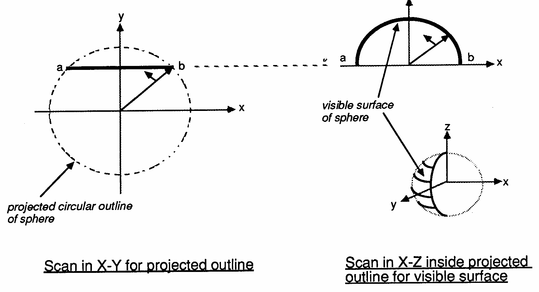
Polygons can be scanned easily since they are planar, and z can be interpolated linearly over planar surfaces. Spheres are not so simple. There are two problems: first, scan converting the sphere involves determining the projected circular outline of the sphere on the screen; secondly, scanning the region inside the outline to compute z and colour at each pixel covered by the sphere. In fact a sphere in perspective does not always project exactly into a circle, but in general this is a close enough approximation. The spheres code was written to allow complex molecules to be rendered. When displaying molecules, the individual atoms are generally small in relation to the complete image, so the distortion due to circular projection is acceptable.
The projected radius of the sphere is obtained from the perspective calculations. Bresenham’s circle algo-rithm [12] is then used to scan the outline of the projected circle, and is also used at each scanline to scan the sphere in z (Figure 5.1). Exact spherical shading is complex (and therefore slow), requiring lots of maths at each pixel (including square roots), so an approximate shading technique is used as described by Fuchs et al. [14]. The visible hemisphere is shaded as though it were a paraboloid. The resulting shading is smooth and very hard to distinguish from correct spherical shading.
| Figure 5.1: Scan
conversion of spheres via Bresenham’s algorithm
|
Scan conversion with a DDA
Scan-converters are generally implemented using a digital differential analyser (DDA), or a variant of Bresenham’s line-drawing algorithm [11, Chapter 2]. The reasoning behind this is that divisions can be avoided, and all addition operations are on integers, improving performance. Tracking an edge with a DDA involves maintaining two items of information about the edge: the current position and the current error term. A step is taken along the ‘driving axis’, the axis of greatest step. A fixed value is unconditionally added to the error term. When the error term overflows (generally this means when the error becomes positive), a step is taken along the ‘driven axis’, and a different fixed value is subtracted from the error term.
Here is an example of drawing a line using Bresenham’s algorithm – it is assumed the deltaX is greater than deltaY, so x is the driving axis:
e = (2 * deltaY) – deltaX;
for (i = 1; i = deltaX; i++)
  {
   plot (x, y);
  e = e + (2 * deltaY);
  if (e > 0)
    {
    y = y + 1;
    e = e – (2 * deltaX);
   X =  X + 1;
  }
Note that a decision must be made at each pixel, the if statement means that the processor will execute a conditional jump instruction. The break in instruction pipelining (and subsequent forced instruction fetch) this causes will consume valuable processor cycles.
Scan conversion on transputers
There is an alternative solution for the transputer. Bresenham’s algorithm removed division operations because historically this was a prohibitively slow operation. The division was removed at the expense of generality – the slope of the line must be between zero and one. This means that a scan converter, which must have y as the driving axis, still requires at least one division operation and also requires greater complexity in the inner loop.
As a division is now necessary, an alternative approach was looked for. The transputer’s designers were sufficiently far-sighted to include fast extended arithmetic operations in the instruction set. Instead of maintaining an error term (which is scaled in terms of deltaX and deltaY, rather than machine precision) we simply put a 32 bit fraction on the end of the 32 bit integer, and use longadd instructions to step along the slope.
The value slope := deltaX / delta Y is computed as a signed 64 bit value (32 integer plus 32 fraction bits), and the if at every pixel is avoided. Computing the slope to 64 bits consumes about 100 processor cycles (5 us) per edge, but simplifying the code in the inner loop makes the fractional version run some 40% faster than the Bresenham version. The code also becomes more readable, as shown in the simplified example below:
y := y + slope -- slope is 64 bits (integer + fraction)
is more obvious than
SEQ
  y: = y + dyBydx	-- dyBydx is the integer part of the slope
  e = e + (2 * deltaY)
  IF
    e > 0	-- take care of fractional part of slope
      SEQ
        y:=y+ 1
        e: = e – (2 * deltaX)
    TRUE
      SKIP
This becomes even more apparent when several variables are being interpolated (i.e. x, z and colour). Note that for x and colour, a 32 bit value for the slope (16 bits integer and 16 bits fraction) would provide sufficient resolution and be faster to compute. However, the advantages of this are outweighed by having to extract the upper 16 bits of the word which contain the desired x and colour values.
The scan conversion of spheres is also done using long arithmetic.
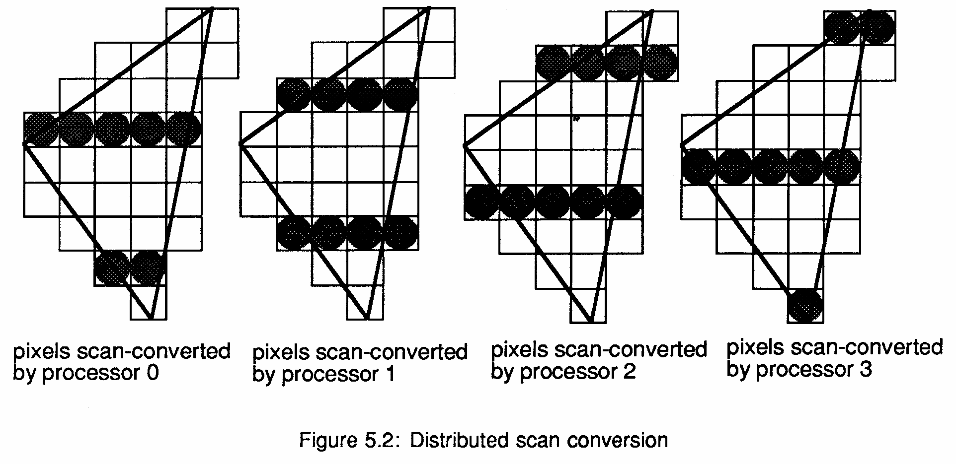
A standard scan converter traverses each polygon one scanline at a time. The distributed scan converter running on N transputers traverses each polygon N lines at a time. Each scan converter starts scanning at a different scanline, i.e. at the lowest y-coordinate enclosed by the polygon which can contribute to its subsection of the image.
In effect, each scan converter reconstructs a slightly different ‘squashed’, but interleaved, copy of the scene. When merged these sub-images create the final picture, so the net effect is that the polygon is fully shaded and Z-buffered (Figure 5.2).
This requires careful coding (and a little more computation) to initiate the scan conversion process and to follow corners correctly, but the scan converter distributed on N machines runs (very nearly) N times as fast as on one machine.
| Figure 5.2: Distributed
scan conversion
|
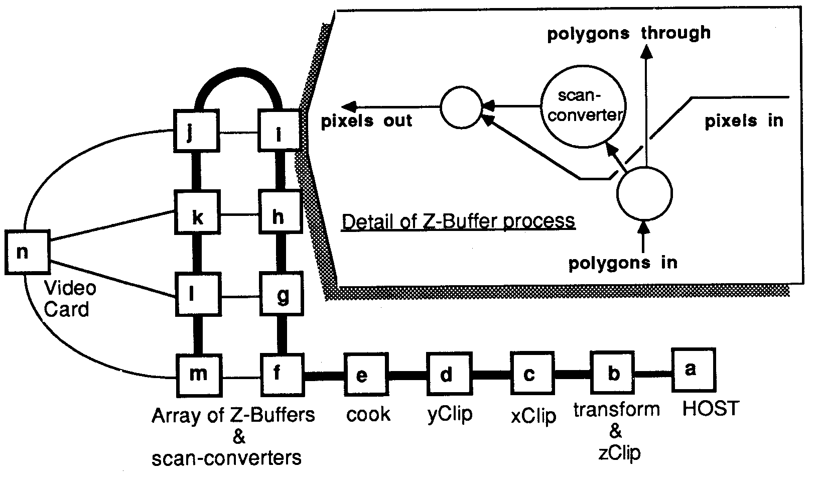
The architecture of the Z-buffer system (Figure 5.3) is simple, but is flexible and easily extended, see Figure 5.3. An INMOS IMS B004 board (a) is used as a database, file interface and user interface. It sends transformation matrices, polygons and spheres to the geometry system.
The geometry system consists of four transputers on a single IMS B003-2 transputer evaluation board, which has been modified by replacing one of the IMS T414-20s with an IMS T800-20. This transputer (b) performs all the floating point computation, performing 3-D transformation, z clipping and conversion to screen coordinates. Two IMS T414s (c and d) then perform x and y clipping. A final IMS T414 (e) preprocesses (‘cooks’) polygons and spheres into a form suitable for the scan converters: polygon vertex format is converted to edge format and edge slopes are computed; coefficients are calculated for the sphere shading equation.
The ‘cooker’ outputs its processed polygons and spheres to the Z-buffer array (f through m). Note the link usage – polygons are passed through the emboldened vertical links, independently of the horizontal links which pass pixels to the graphics card (n). This separation of polygon flow and pixel flow allows a finished frame to be passed to the graphics card while the next frame is being computed, pipelining work efficiently for animated sequences. This organisation also takes maximum advantage of the autonomous link engines on each transputer. The graphics card used is an IMS B007 evaluation board which has 2 banks of video memory allowing the next frame to be read in without disturbing the currently displayed image. When the complete frame has been received the two memory banks are swapped by writing to a control register. This must be synchronised with the frame flyback of the display to avoid distracting visual artefacts.
| Figure 5.3: Distributed
Z-buffer architecture
|
The Z-buffer is fully interactive, and on our existing models image generation speeds range from over 10 frames per second down to around 1 frame per second.
Performance of the system is sensitive to the number of polygons and to screen coverage per polygon. With small numbers of large polygons, scan conversion time dominates, so a larger number of scan converters gives a linear performance improvement.
The IMS T800 in the geometry system is crucial for images with large numbers of small polygons. In this case screen coverage and hence scan conversion time (per polygon) is low, and transformation time can dominate unless a lot of floating point performance is available. If the IMS T800 is replaced by an IMS T414, refresh rates can drop by a factor of 15 for a complex model such as that of the IMS T800 package.
Some screen photographs of the output generated by this system are included at the front of this note. The bevelled cubes consist of 112 polygons, 128 points, and were computed at 8.4 frames per second using 8 scan converters. The molecule (54 spheres, 108 points) achieves 6.3 frames per second, but this drops dramatically if the screen coverage is increased, since the computation per pixel is higher for spheres than for polygons. Note that the individual atoms intersect correctly, and that the lighting conditions are locally modelled – the highlight is in different positions on different atoms. The Starship Enterprise (596 polygons, 943 points) is displayed at 2.8 frames per second; no surface normal information is yet available for this model, so it is flat shaded. The IMS T800 package (1254 polygons, 1584 points) refreshes at between 1.8 and 1.4 frames per second.
The INMOS flight simulator came from the need to demonstrate the real time graphics capabilities of the transputer family. Although the Z-buffer is much faster than any other yet implemented on microprocessors (rather than custom hardware), it is still not fast enough to implement the vision system of a flight simulator, even when running with thirty two scan converters. This is due to the per pixel calculation involved in 2-buffering – a ‘greater than’ comparison is required at every pixel covered by each polygon. An alternative hidden surface algorithm without this overhead is required for the flight simulator.
The primary requirement of the flight simulator was that it be fast. It should be able to sustain 17 frames per second, the bandwidth limit into the IMS B007 graphics card, when shading a reasonable number of polygons – say 200 to 300. It should have low latency, i.e. the time from user input to visual feedback should be no more than three, preferably only two frame times. It should also use only a small number of transputers to implement a four player system.
The core of the flight simulator is a distributed polygon shader, similar in design to the scan converter in the Z-buffer. It is optimised for flat shading of polygons and does not include the Z-buffer. This reduces the amount of computation and means that a fast block move operation can be used to shade the horizontal regions between polygon edges. It can be arranged that the block move copies the value defining the colour from on-chip memory so a 32 bit word can be copied (in other words, four pixels can be shaded) every n+1 machine cycles, where n is the number of machine cycles required to access off-chip memory.
When coded in this way, a 20MHz transputer with single wait-state (4 cycle) external memory can shade polygons at a rate of 16 million 8 bit pixels per second, or 62.5 nanoseconds per pixel. Four transputers can therefore shade at up to 64 million pixels per second, only 15.6 nanoseconds per pixel. With this high polygon shading speed it becomes possible to display a reasonable number (over 200 ‘average size’) polygons at 17 frames per second, a very high number for a software implementation with no custom hardware. Using four transputers allowed the use of the INMOS IMS 8003-2 transputer evaluation board, so no new hardware design was necessary.
From the previous figures quoted for transformation time, the IMS T800 has processing power to spare, it can transform 200 quadrilaterals (800 points) in less than one sixtieth of a second. Three more transputers are used in the geometry system – another IMS T800 for z clipping (often called hither and yon clipping) and conversion to screen coordinates, and two IMS T414s for clipping in x and y. Clipping in x and y are performed in screen space, so integer maths is sufficient. The geometry system now consists of four transputers, so again an IMS B003-2 is used, but this time slightly modified (two IMS T414s replaced with IMS T800s).
At this stage the importance of pin compatibility between the IMS T414 and IMS T800 cannot be over emphasised – it allows high floating point performance to be injected into a multiprocessor system just where it is required, allowing performance tuning simply by removing one transputer from a socket and plugging in another.
This is a very fast polygon shader and geometry system, all that is required is a hidden surface algorithm which outputs its solution in polygon form to implement the entire vision system of the flight simulator.
The BSP-tree [13] is a recursive data structure which implicitly holds all possible hidden surface solutions for the object it represents. Each node of the BSP-tree contains a polygon and pointers to front and back subtrees. The front subtree contains all polygons in front of the node polygon, the back subtree contains those behind the node polygon. The notion of ‘in front-ness’ is determined by substitution of the current viewing position into the plane equation of the polygon.
By traversing the BSP-tree in an order determined solely by
the viewing position, the polygons are passed to the distributed
polygon shader in reverse z order, so that nearer surfaces are
painted after (and hence obscure) more distant surfaces, giving
the correct hidden surface solutiom.
The following algorithm is used to perform BSP-tree traversal:
traverseTree (tree)
{
  if (tree is empty)
    return
  else
  {
    if (view point in front of rootPolygon)
    {
      traverseTree (tree->back);
      displayPolygon (tree->rootPolygon);
      traverseTree (tree->front);
    }
    else
    {
      traverseTree (tree->front);
      displayPolygon (tree->rootPolygon);
      traverseTree (tree->back);
    }
  }
}
In some applications this procedure can be optimised by not painting backfacing polygons. This is useful if there are only closed objects in the model, for example a cube has six faces but only three of these are visible at any time. In the flight simulator each polygon has a flag to indicate whether it should be painted when the viewpoint is behind it. This allows rotor blades, for example, to be implemented as a single polygon while allowing back face elimination on the body of the helicopter.
This process is recursive – our traverser is implemented in occam which does not allow recursive procedure definitions, so a state machine is constructed. Further details of implementing recursive data structures and procedures in OCCGFl programs can be found in another INMOS technical note [8]. The state machine maintains two variables, the current node in the tree, and the current action being performed. These nodes and actions are explicitly stacked as the tree is traversed. Here is an outline of the state machine in occam:
SEQ
  -- initialise
  push (NIL, a.terminate)
  action := a.testPosition
  node := rootNode
  WHILE action <> a. terminate
    CASE action

      a.testPosition
      -- test whether we are in front of
      -- or behind the current polygon
    IF
      node = NIL
        -- end of subtree
        pop (node, action)
      inFront (node, viewPoint)
      -- in front of current polygon
    SEQ
      push (node, a.traverseFront)
      node := tree[node + backSubTree]
      TRUE
        -- behind current polygon
        SEQ
        push (node, a.traverseBack)
        node := tree[node + frontSubTree]

     a.traverseFront
      -- output current polygon
      -- then traverse front subtree
      SEQ
        outputPoly (node)
        action := a.testPosition
        node := tree[node + frontSubTree]

    a.traverseBack
      -- output current polygon
      -- then traverse back subtree
      SEQ
        outputPoly (node)
        action := a.testPosition
        node := tree[node + backSubTree]
Only half a dozen floating point instructions are required to determine which subtree to traverse first at any node, so the BSP-tree traverser was incorporated into the same transputer as the 3-D transformation, leaving run time still dominated by polygon painting time.
BSP-trees are used to determine polygon visibility within each object in the simulator (e.g. aeroplanes, helicopters, teapots, buildings), and a simple bounding box test in z is used to determine the relative z ordering of objects. This means that the system will not correctly render objects when they intersect. However, if this condition occurs in the flight simulator it implies that the objects have collided.
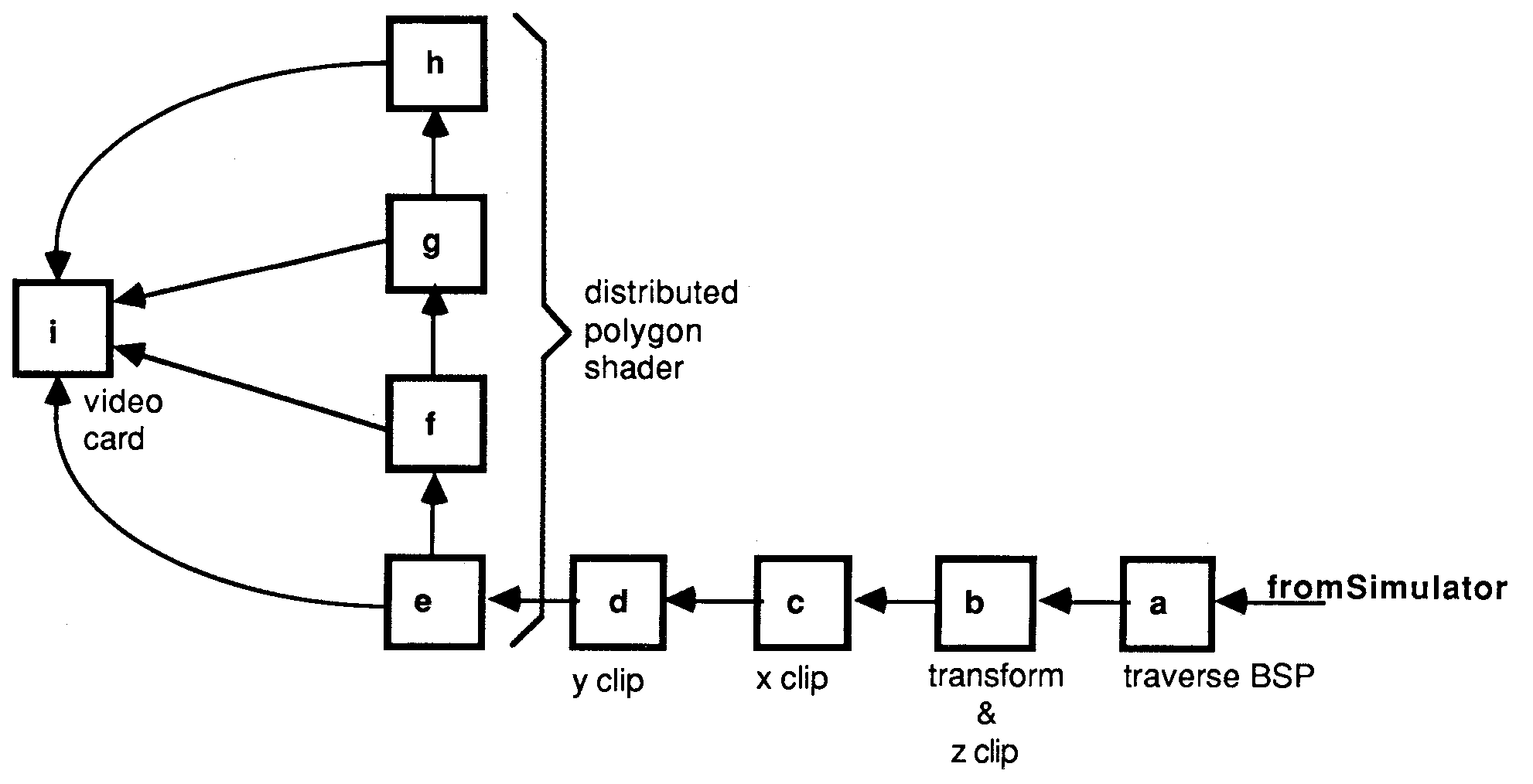
The vision system of the flight simulator is as illustrated below (Figure 6.1). A geometry system consisting of four transputers performs: (a) BSP-tree traversal and 3-D transformation; (b) z clipping and conversion to screen coordinates; (a) y clipping; and (d) x clipping.
Four transputers (d, e, f and g) perform distributed polygon shading and a graphics card operates as a pixel sink (h). The processor in the graphics card would normally be idle, the transputer simply waiting for images to appear down its links. This is a waste of a good processor, so more functionality is added. The graphics card now implements a head up display showing an artificial horizon, air speed, altitude, bearing, radar with enemy positions and missile fuel readings. All of these make extensive use of the IMS T800’s 2-D move instructions.
| Figure 6.1: Flight
simulator vision system
|
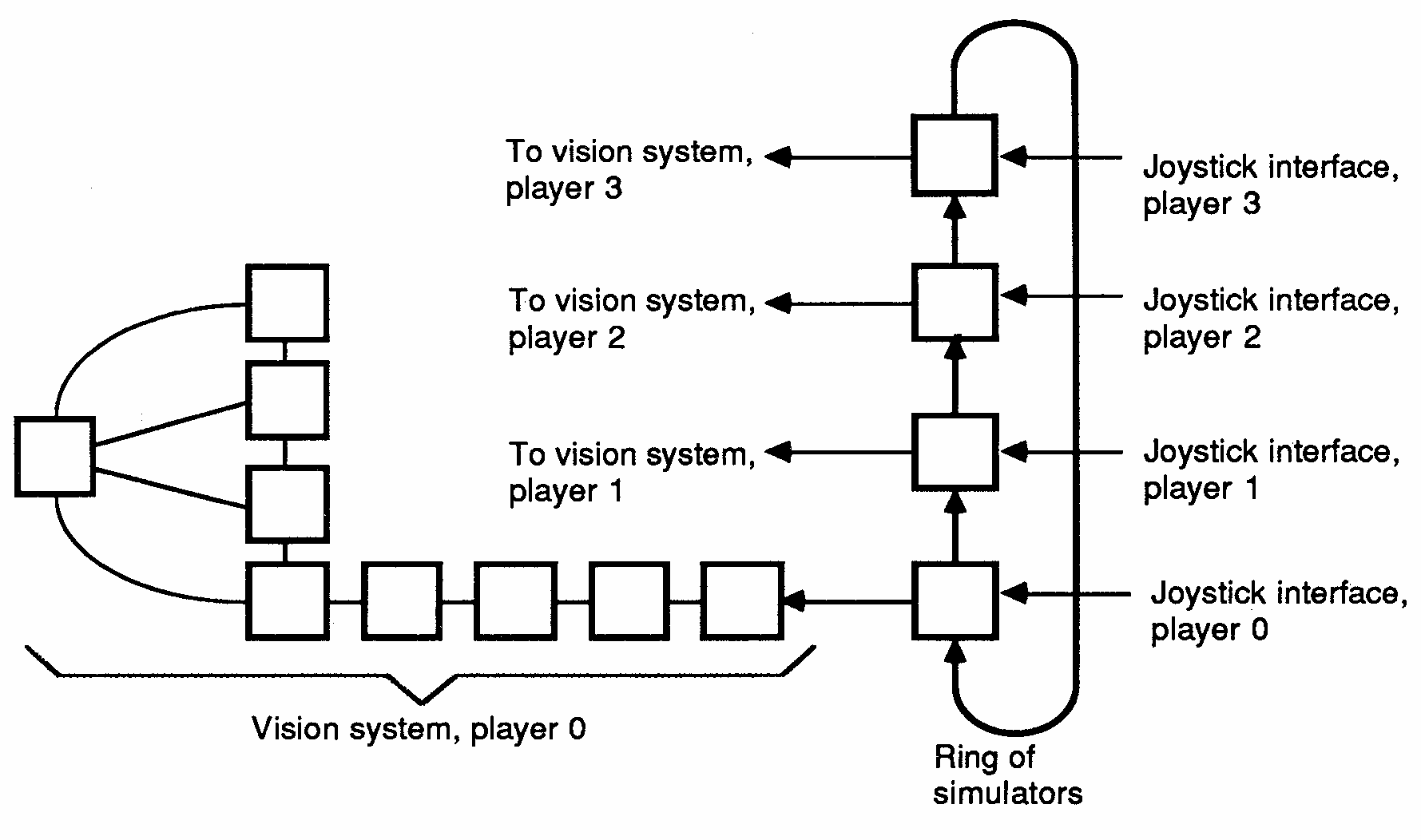
The simulator itself runs on a single transputer with the vision system connected to one link, and has been designed to allow many simulators to be connected in a ring (Figure 6.2). This allows a number of players to take part in a combat simulation, each player seeing the others through his simulated cockpit window.
At SIGGRAPH ’87 members of the INMOS Late Night Rendering Crew demonstrated a four player combat simulator, and members of the public were invited to try and shoot down INMOS application engineers. The whole system (i.e. four entire flight simulators) was housed in a pair of INMOS card cages; taking up only 13 double extended eurocard slots and less than five cubic feet. In the course of a 10 hour combat session more than a terabyte of data (i.e. over a thousand gigabytes) will flow through a four player simulator.
The implementation of the flight simulator is described in greater detail in another INMOS technical note [7].
The flight simulator performs as well as anticipated – it consistently achieves a refresh rate of 17 frames per second. The main limiting factor is the need to synchronise the updates to the graphics display with frame flyback. Frame rates approaching the theoretical maximum of 27 frames per second could be achieved by having more buffering in the graphics display hardware. This would allow image data to be received asynchronously with frame flyback. If desired even higher frame rates can be obtained by using more than one transputer in the display system.
Included at the front of this note are some stills from the flight simulator. These images only come to life when animated at 17 frames per second. The impression of flight is uncanny, despite the simplistic polyhedral design of the aircraft.
A final word on the flight simulator – the distributed scan converter and the BSP-tree traverser had been written for previous example programs, but the rest of the system was written, debugged and functioning in only two weeks. In fact, since the author of the rest of the simulator is an INMOS Field Applications Engineer, ail his work was done in evening and weekend stints, as he is on the road most weekdays. We believe this is a record.
| Figure 6.2: Full four
player simulator
|
The IMS T800 offers all the features required for high performance computer graphics. It is a very high performance microprocessor capable of being used in large numbers to form extremely powerful multiprocessor computers, with a few well chosen instructions for computer graphics support.
The IMS T800s 2-D block manipulation instructions make it an ideal candidate for the next generation of high resolution full colour workstations, and for future generations of colour laser printer controllers.
The IMS T800 has sufficient floating point performance for any application. If more than 1.5 MFLOPS are required then use more transputers. Thirty two IMS T800-20s offer the computational equivalent of current vector supercomputers (48 consistently achievable MFLOPS), take up only 56 square inches of PCB area (i.e. they will fit on an IBM PC plug in card), and at current prices (January 1988) cost less than £20,000.
[1] Transputer reference manual
INMOS Limited
Prentice Hall
ISBN 0-13-929001-X
[2] occam reference manual
INMOS Limited
Prentice Hall
ISBN 0-13-629312-3
[3] IMS T800 architecture
Technical Note 6
INMOS Limited
[4] Exploiting concurrency: a ray tracing example
Technical Note 7
INMOS Limited
[5] Notes on graphics support and performance improvements on
the IMS T800
Technical Note 26
INMOS Limited
[6] Lies, damned lies and benchmarks
Technical Note 27
INMOS Limited
[7] The INMOS flight simulator
Technical Note 36
INMOS Limited
[8] Data structures and recursion in occam
Technical Note 38
INMOS Limited
[9] A transputer based distributed graphics display
Technical Note 46
INMOS Limited
[10] The transputer instruction set: a compiler writers guide
INMOS Limited
[11] Principles of interactive computer graphics
William M. Newman R Robert F. Sproull
McGraw Hill
[12] A linear algorithm for incremental digital display of
circular arcs
J.E. Bresenham
CACM 20(2):100-106, February 1977
[13] Near real-time shaded display of rigid objects
Fuchs, Abram 8 Grant
Computer Graphics 17(3), July 1983 (Proc. SIGGRAPH 83)
[14] Fast spheres, shadows, textures, transparencies and image
enhancements in Pixel-Planes
Fuchs, Goldfeather, Hultquist, Spach, Austin, Brooks, Eyles and
Poulton
Computer Graphics 19(3), July 1985 (Proc. SIGGRAPH 85)
[15] Reentrant polygon clipping
Ivan E. Sutherland & Gary W. Hodgman
CACM 17(1), January 1974
March 1988
72 APP 037 00